Clasificadores
The slides are available here!
K-Nearest Neighbors (K-NN)
Overview
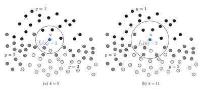
K-Nearest Neighbors (K-NN) is an instance-based learning algorithm that classifies a new point based on the majority label among its K closest training examples in the feature space. It does not build an explicit model.
Classification Rule
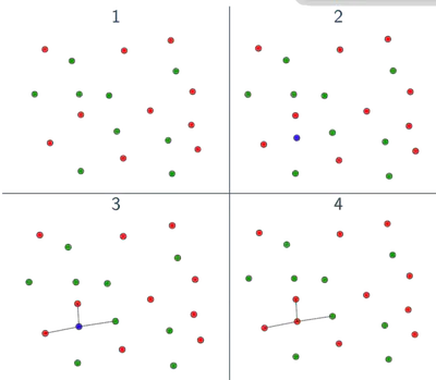
Given a point \( \mathbf{X} \), the K-NN classifier performs the following:
- Let \( S = \{(\mathbf{X}_i, y_i)\}_{i=1}^n \) be the training set
- Define a distance metric \( d(\cdot, \cdot) \)
- Sort the training points by distance to \( \mathbf{X} \)
- Take the first \( K \) elements: \( S^K_\mathbf{X} = \{\mathbf{X}_{\sigma(1)}, \dots, \mathbf{X}_{\sigma(K)}\} \)
- Count occurrences of each label in this subset
Where \( N^K_y(\mathbf{X}) \) is the number of neighbors with label \( y \).
Choosing K
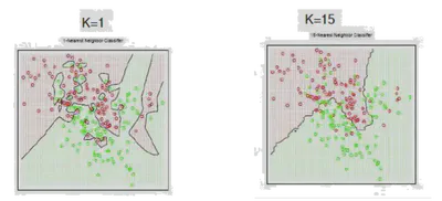
The hyperparameter \( K \) controls the bias-variance tradeoff:
- Small \( K \) (e.g., 1 or 3): Low bias, high variance; very sensitive to noise.
- Large \( K \) (e.g., 20+): High bias, low variance; smooths out decision boundary.
Distance Metrics
The choice of distance metric can significantly affect K-NN performance. Common metrics include:
\[ d(x, y) = \left( \sum_i |x_i - y_i|^p \right)^{1/p} \]- Manhattan distance: \( p=1 \)
- Euclidean distance: \( p=2 \)
- Chebyshev distance: \( p = \infty \)
- Mahalanobis distance: Takes into account feature covariance: \[ d(x, y) = \sqrt{(x - y)^T \Sigma^{-1} (x - y)} \]
Important: Normalize your features. Otherwise, features with large numeric ranges can dominate the distance computation.
More: Scikit-learn distance metrics
Feature Scaling and Normalization
Before using K-NN, apply proper preprocessing:
Standardization: Gaussian distribution with zero mean and unit variance
\[ x' = \frac{x - \mu_x}{\sigma_x} \]Min-Max Scaling: Scale to \([0,1]\)
\[ x' = \frac{x - \min(x)}{\max(x) - \min(x)} \]L2 Normalization: Unit vector (used when orientation is more important than magnitude)
More on preprocessing: scikit-learn documentation
Strengths and Limitations
Advantages:
- Simple and intuitive
- No training time (lazy learner)
- Adapts to non-linear boundaries
Limitations:
- Computationally expensive at test time
- Suffers from the curse of dimensionality: as dimensionality increases, all distances converge
- Sensitive to irrelevant features
Naive Bayes
Bayes’ Rule
Bayes’ theorem relates the posterior probability of a class to its prior and likelihood:
\[ P(c|o) = \frac{P(o|c) \cdot P(c)}{P(o)} \]Where:
- \( P(c) \): prior probability of class \( c \)
- \( P(o|c) \): likelihood of observation given the class
- \( P(o) \): evidence (can be ignored for classification)
- \( P(c|o) \): posterior
Naive Assumption
Naive Bayes assumes that features are conditionally independent given the class:
\[ P(o|c) = \prod_{i=1}^d P(x_i | c) \]Thus:
\[ \hat{c} = \arg\max_c P(c) \cdot \prod_{i=1}^d P(x_i | c) \]This assumption is rarely true in real-world data, but the algorithm often performs well despite it.
Parameter Estimation
For categorical features:
\[ P(x_i = v | c) = \frac{\text{count}(x_i = v, c)}{\text{count}(c)} \]Laplace Smoothing
If a word/feature is not observed in class \( c \), then \( P(x_i | c) = 0 \), which will nullify the whole product. Laplace smoothing fixes this:
\[ P(x_i = v | c) = \frac{\text{count}(x_i = v, c) + \alpha}{\text{count}(c) + \alpha \cdot n} \]- \( \alpha \): smoothing parameter (usually 1)
- \( n \): number of possible values of \( x_i \)
Continuous Features: Gaussian Naive Bayes
If features are continuous, assume they follow a Gaussian distribution per class:
\[ P(x_i | y) = \frac{1}{\sqrt{2\pi \sigma^2_y}} \exp\left( -\frac{(x_i - \mu_y)^2}{2\sigma^2_y} \right) \]Estimate \( \mu_y \) and \( \sigma_y \) from training data using MLE.
Pros and Cons
Pros:
- Very fast to train
- Robust to irrelevant features
- Works well with high-dimensional, sparse data (e.g., text classification)
Cons:
- Strong independence assumption is rarely true
- Poor probability estimates (outputs not well-calibrated)
Decision Trees
Overview
Decision Trees split the feature space using axis-aligned hyperplanes to partition data into regions that are homogeneous in class labels.
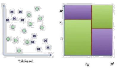
Each internal node splits on one feature. Each leaf represents a class.
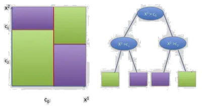
- Use axis-aligned splits \( x^j = \tau \)
- Represent decision process in a binary tree
- Each node corresponds to a split
Where each \( \mathcal{C}_l \) is a region defined by a set of splits, and \( \alpha_l \) is the label for that region.
Tree Construction
At each node, the tree:
- Selects a feature \( x^j \) and a threshold \( \tau \)
- Divides the data into:
- Left: \( \{x \in \mathcal{S} \mid x^j \leq \tau\} \)
- Right: \( \{x \in \mathcal{S} \mid x^j > \tau\} \)
It chooses the best split by minimizing the impurity.
Impurity Measures
Given a subset \( \mathcal{S} \), define class proportions \( p_c \). Common criteria:
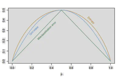
Entropy:
\[ H(\mathcal{S}) = -\sum_c p_c \log p_c \]Gini Index:
\[ H(\mathcal{S}) = \sum_c p_c(1 - p_c) \]Classification Error:
\[ H(\mathcal{S}) = 1 - \max_c p_c \]
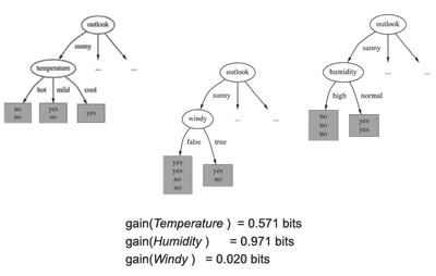
Information Gain
Choose the feature \( j \) and threshold \( \tau \) that minimize:
\[ L(t_{j,\tau}, \mathcal{S}) = \frac{|\mathcal{D}|}{n} H(\mathcal{D}) + \frac{|\mathcal{I}|}{n} H(\mathcal{I}) \]Where \( \mathcal{D} \) and \( \mathcal{I} \) are the left and right splits.
The Information Gain is the reduction in entropy from the split.
Stopping Criteria
A tree stops growing when:
- Max depth is reached
- Leaf nodes have fewer than a minimum number of samples
- All samples in a node belong to the same class
Be cautious: allowing unrestricted growth leads to overfitting.
Ensemble Methods
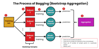
Bagging (Bootstrap Aggregation)
Bagging is an ensemble method where:
- Multiple models are trained on different bootstrap samples
- Their outputs are aggregated (majority vote or average)
Reduces variance, making the model more stable.
Equation for MSE:
\[ MSE(f_{ens}) = \frac{1}{T^2} \mathbb{E}\left[ \left( \sum_t \epsilon_t(x) \right)^2 \right] \]If \( \epsilon_t \) are uncorrelated, variance is reduced.
Boosting
Boosting trains models sequentially, each correcting its predecessor’s mistakes:
- Initialize equal weights on data
- Train model \( h_t \)
- Increase weights on misclassified examples
- Aggregate predictions with weighted votes
Common boosting algorithms: AdaBoost, Gradient Boosting
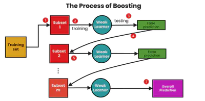
Boosting Example
Binary classifiers are trained and added together:
\[ F_n(x) = \text{sign}(H_{n-1}(x) + h_n(x)) \]Each learner focuses more on points misclassified by the previous.
🔗 More on Boosting
🔗 Adaboost from Jiri Matas class
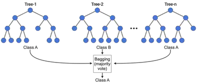
Random Forest
Motivation
Decision trees are high-variance models. A small change in data can lead to very different trees.
Random Forests reduce variance by averaging multiple decision trees trained on different subsets of the data and features.
Algorithm
- For each tree \( t \in 1..T \):
- Sample \( \mathcal{S}^{(t)} \) using bootstrap (sample with replacement)
- Randomly choose \( k \ll F \) features at each node
- Train a decision tree \( h^{(t)} \)
- Output prediction: \[ h^{(T)}(x) = \frac{1}{T} \sum_t h^{(t)}(x) \]
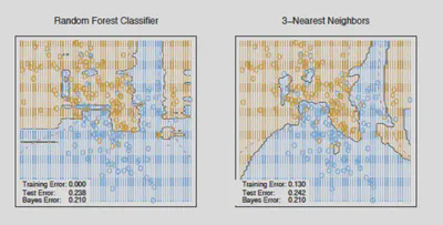
Decision Boundaries
Random Forest Regression
For regression tasks, replace impurity by variance reduction:
\[ L(t_{j, \tau}, \mathcal{S}) = VAR(\mathcal{S}) - \frac{|\mathcal{D}|}{n} VAR(\mathcal{D}) - \frac{|\mathcal{I}|}{n} VAR(\mathcal{I}) \]Where:
\[ VAR(\mathcal{S}) = \frac{1}{|\mathcal{S}|} \sum_{(x^i, y^i) \in \mathcal{S}} (y^i - \bar{y})^2 \]Summary Tables
Strengths and Weaknesses
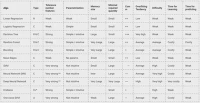
- K-NN: Easy to use, but slow and sensitive to irrelevant features
- Naive Bayes: Fast, works well with text
- Decision Trees: Interpretable, prone to overfitting
- Random Forests: Powerful and stable, but harder to interpret
🔗 SAP ML algorithms summary
🔗 Google Sheet: model comparison
Model Selection Flow
You can refer to the scikit-learn decision flow:
